beginning econometrics

Overview:

Watch

Introduction To Stationary And Non-Stationary Processes

Introduction To Stationary And Non-Stationary Processes

Financial institutions and corporations as well as individual investors and researchers often use financial time series data (such as asset prices, exchange rates, GDP, inflation and other macroeconomic indicators) in economic forecasts, stock market analysis or studies of the data itself.

But refining data is key to being able to apply it to your stock analysis. In this article, we'll show you how to isolate the data points that are relevant to your stock reports.

Cooking Raw Data
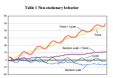
Data points are often non-stationary or have means, variances and covariances that change over time. Non-stationary behaviors can be trends, cycles, random walks or combinations of the three.

Non-stationary data, as a rule, are unpredictable and cannot be modeled or forecasted. The results obtained by using non-stationary time series may be spurious in that they may indicate a relationship between two variables where one does not exist. In order to receive consistent, reliable results, the non-stationary data needs to be transformed into stationary data. In contrast to the non-stationary process that has a variable variance and a mean that does not remain near, or returns to a long-run mean over time, the stationary process reverts around a constant long-term mean and has a constant variance independent of time.

Figure 1

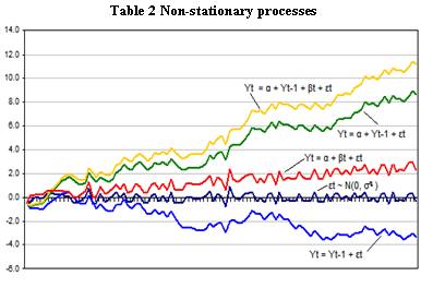
Types of Non-Stationary ProcessesBefore we get to the point of transformation for the non-stationary financial time series data, we should distinguish between the different types of the non-stationary processes. This will provide us with a better understanding of the processes and allow us to apply the correct transformation. Examples of non-stationary processes are random walk with or without a drift (a slow steady change) and deterministic trends (trends that are constant, positive or negative, independent of time for the whole life of the series).

Figure 2

• Pure Random Walk (Y_t = Y_t-1 + ε_t )Random walk predicts that the value at time "t" will be equal to the last period value plus a stochastic (non-systematic) component that is a white noise, which means ε_t is independent and identically distributed with mean "0" and variance "σ²". Random walk can also be named a process integrated of some order, a process with a unit root or a process with a stochastic trend. It is a non mean reverting process that can move away from the mean either in a positive or negative direction. Another characteristic of a random walk is that the variance evolves over time and goes to infinity as time goes to infinity; therefore, a random walk cannot be predicted.
• Random Walk with Drift (Y_t = α + Y_t-1 + ε_t )If the random walk model predicts that the value at time "t" will equal the last period's value plus a constant, or drift (α), and a white noise term (ε_t), then the process is random walk with a drift. It also does not revert to a long-run mean and has variance dependent on time.
• Deterministic Trend (Y_t = α + βt + ε_t )Often a random walk with a drift is confused for a deterministic trend. Both include a drift and a white noise component, but the value at time "t" in the case of a random walk is regressed on the last period's value (Y_t-1), while in the case of a deterministic trend it is regressed on a time trend (βt). A non-stationary process with a deterministic trend has a mean that grows around a fixed trend, which is constant and independent of time.
• Random Walk with Drift and Deterministic Trend (Y_t = α + Y_t-1 + βt + ε_t ) 
  Another example is a non-stationary process that combines a random walk with a drift component (α) and a deterministic trend (βt).It specifies the value at time "t" by the last period's value, a drift, a trend and a stochastic component. (To learn more about random walks and trends, see our Financial Concepts tutorial.)

Trend and Difference StationaryA random walk with or without a drift can be transformed to a stationary process by differencing (subtracting Y_t-1 from Y_t, taking the difference Y_t - Y_t-1) correspondingly to Y_t - Y_t-1 = ε_t or Y_t - Y_t-1 = α + ε_t and then the process becomes difference-stationary. The disadvantage of differencing is that the process loses one observation each time the difference is taken.

Copryright © 2007 Investopedia.com

Figure 3

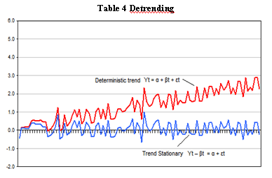
A non-stationary process with a deterministic trend becomes stationary after removing the trend, or detrending. For example, Yt = α + βt + εt is transformed into a stationary process by subtracting the trend βt: Yt - βt = α + εt, as shown in Figure 4 below. No observation is lost when detrending is used to transform a non-stationary process to a stationary one.

Figure 4

In the case of a random walk with a drift and deterministic trend, detrending can remove the deterministic trend and the drift, but the variance will continue to go to infinity. As a result, differencing must also be applied to remove the stochastic trend.

ConclusionUsing non-stationary time series data in financial models produces unreliable and spurious results and leads to poor understanding and forecasting. The solution to the problem is to transform the time series data so that it becomes stationary. If the non-stationary process is a random walk with or without a drift, it is transformed to stationary process by differencing. On the other hand, if the time series data analyzed exhibits a deterministic trend, the spurious results can be avoided by detrending. Sometimes the non-stationary series may combine a stochastic and deterministic trend at the same time and to avoid obtaining misleading results both differencing and detrending should be applied, as differencing will remove the trend in the variance and detrending will remove the deterministic trend.